Variable Selection: The Secret Weapon for Powerful Predictive Models

Variable selection is a crucial step in building effective machine learning models. It involves choosing the ‘best’ subset of predictors or features to include in the model. The goal is to identify the most relevant variables that will improve the model’s performance and accuracy. By carefully selecting these variables, we can enhance the model’s predictive power and efficiency.

Parsimony in variable selection is paramount in constructing effective models. It emphasizes the balance between model simplicity and explanatory power. The Adjusted-R^2 concept (everyone may be familiar with) complements this by adjusting the goodness-of-fit measure to account for the number of variables used, providing a more accurate reflection of model performance. On the flip side, the curse of dimensionality warns against including an excessive number of variables, which can lead to overfitting and diminish the model’s predictive capability. Striking a balance between these factors ensures that models are both interpretable and robust, capturing essential relationships without unnecessary complexity

Below are robust steps we can try for variable selection in model pipeline

Step 1: Preliminary Filtering

Preliminary filtering is the process of quickly and independently screening variables to assess their individual relevance, regardless of any machine learning model. In essence, it helps filter out irrelevant variables.

• Non-Zero Variance: This filter removes features with constant values (zero variance) because they provide no useful information. In other words, if the concentration of a particular value within a variable is too high, that variable is considered to have low information content and should be removed.

• Predictive Power Score (PPS): PPS is a more robust and powerful alternative to traditional correlation. It only considers the magnitude of the relationship, not the direction, and ranges from 0 (no predictive power) to 1 (perfect predictive power). PPS is data-type agnostic, meaning it can work with both categorical and numerical data. Its biggest advantage is the ability to detect asymmetric, non-linear relationships.

PPS with ‘hmeq’ dataset:

• Marginal Information Value (MIV): MIV calculates the incremental IV gain by adding a new variable to an existing set of variables. In contrast to traditional IV, which ranks variables based solely on individual importance, MIV guides feature selection by iteratively adding features that maximize information gain. Traditional IV may inadvertently introduce collinear variables, whereas MIV seeks variables that improve the model’s predictive power without introducing collinearity. MIV is typically calculated in a stepwise manner (but still be considered as filter in my opinion), starting with an initial model and iteratively adding features with the highest MIV until no further improvement is observed.

Step 2: Stepwise Selection

Wrapper selection further refines the feature set by evaluating combinations of features and selecting the best-performing subset. With the wrapper selection method, you can build a model with a parsimonious set of highly relevant features that collectively have high predictive power.

• Recursive Feature Elimination (RFE): RFE is a wrapper method that starts with all features and iteratively removes the least important ones. In each iteration, a model is trained on the remaining features, and feature importances are calculated. The least important feature is then removed, and the process is repeated until the desired number of features is reached. While RFE may resemble Stepwise Regression, it is not strictly considered as such. RFE is a backward selection method that uses variable importance scores as criteria (unlike Stepwise, which relies on statistical tests), making it useful in avoiding overfitting. Additionally, RFE’s flexibility allows it to be used with various models, including linear regression, support vector machines, and decision trees.

Step 3: Performance-based Selection

The most common validation performance metric in credit risk models is AUC (Area Under the Receiver Operating Characteristic curve), so this variable selection step can also be called AUC-based selection. It selects the set of variables that directly optimize the AUC-ROC curve. Moreover, it can be extended to use other metrics besides the AUC-ROC curve. Additionally, different estimators (I personally have tried Ranger-a quick Random Forest) other than the original logistic regression can be used in this technique’s procedure.

BART using Ranger with ‘hmeq’ dataset: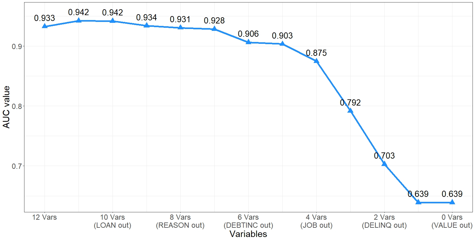

• BART: (BAckward Regression Trimming): This technique was introduced by Professor Bart Baesens, and more information can be found here: https://github.com/MariaOskarsdottir/BART. The procedure is also outlined in the GitHub link. It is also useful for determining the optimal cutoff for the number of variables to include in the model by directly optimizing the chosen performance metric.

**Sample code will follow in different markdown**